Experimental Prediction using a Binding-type and GCN NN Ensembles

This example shows how to predict binding-type and GCN histograms from pdfs

from __future__ import division
import matplotlib.pyplot as plt
import matplotlib.gridspec as gridspec
import numpy as np
from jl_spectra_2_structure import HREEL_2_scaledIR
from jl_spectra_2_structure.plotting_tools import set_figure_settings
from jl_spectra_2_structure.cross_validation import LOAD_CROSS_VALIDATION
from jl_spectra_2_structure import get_exp_data_path

set figure settings

set_figure_settings('paper')

Load cross validation runs and generate neural network ensembles

BINDING_TYPE_PATH = 'C:/Users/lansf/Documents/Data/IR_Materials_Gap/cv_BW/CO_BINDING_TYPE_HIGH'
GCN_PATH = 'C:/Users/lansf/Documents/Data/IR_Materials_Gap/cv_BW/CO_GCN_HIGH'
Downloads = r'C:\Users\lansf\Downloads'
CV_class = LOAD_CROSS_VALIDATION(cross_validation_path=BINDING_TYPE_PATH)
CV_class.load_CV_class(0)
NN_CNCO = CV_class.get_NN_ensemble(np.arange(len(CV_class.CV_FILES)).tolist(),use_all_cv_NN=True)
CV_class_GCN = LOAD_CROSS_VALIDATION(cross_validation_path=GCN_PATH)
NN_GCN = CV_class_GCN.get_NN_ensemble(np.arange(len(CV_class_GCN.CV_FILES)).tolist(), use_all_cv_NN=True)

Load experimental spectra and generate predictions with 95% prediction range

X = np.linspace(CV_class.LOW_FREQUENCY,CV_class.HIGH_FREQUENCY,num=CV_class.ENERGY_POINTS,endpoint=True)
EXP_FILES = np.array(get_exp_data_path())[[3,1,0,2]]
IR_DATA = np.zeros((len(EXP_FILES),X.shape[0]))
for count, file in enumerate(EXP_FILES):
    IR_DATA[count] = HREEL_2_scaledIR(np.loadtxt(file, delimiter=',', usecols=(0, 1)).T, PEAK_CONV = 2.7, frequency_range=X)
Surfaces = ['c4x2Pt111', 'LowCovPt111', 'p1x2Pt110','Ptnano']
NUM_SURFACES = len(Surfaces)
NUM_PREDICTIONS = len(NN_CNCO.NN_LIST)
CNCO_prediction = NN_CNCO.predict(IR_DATA,create_predictions_list=True)
GCN_prediction = NN_GCN.predict(IR_DATA,create_predictions_list=True)
CNCO_sorted = [np.sort(np.array(NN_CNCO.PREDICTIONS_LIST)[:,i,:],axis=0) for i in range(NUM_SURFACES)]
GCN_sorted = [np.sort(np.array(NN_GCN.PREDICTIONS_LIST)[:,i,:],axis=0) for i in range(NUM_SURFACES)]
CNCO_95U = [CNCO_sorted[i][int(0.95*NUM_PREDICTIONS)] - CNCO_prediction[i] for i in range(NUM_SURFACES)]
CNCO_95L = [CNCO_prediction[i]- CNCO_sorted[i][int(0.05*NUM_PREDICTIONS)] for i in range(NUM_SURFACES)]
GCN_95U = [GCN_sorted[i][int(0.95*NUM_PREDICTIONS)] - GCN_prediction[i] for i in range(NUM_SURFACES)]
GCN_95L = [GCN_prediction[i]- GCN_sorted[i][int(0.05*NUM_PREDICTIONS)] for i in range(NUM_SURFACES)]

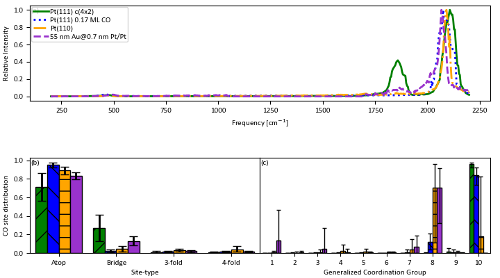
Plot spectra and predictions with 95% prediction range

linestyle = ['-',':','-.','--']
color = ['g','b', 'orange','darkorchid']
G = gridspec.GridSpec(2, 2)
x_offset = [-0.3,-0.1,0.1,0.3]
hatch = ['/','\\','-',None]
G.update(wspace=0.0,hspace=.6)
plt.figure(0,figsize=(7.2,4))
ax3 = plt.subplot(G[0,:])
for i in range(NUM_SURFACES):
    plt.plot(X,IR_DATA[i],color[i],linestyle=linestyle[i])
plt.legend(['Pt(111) c(4x2)','Pt(111) 0.17 ML CO', 'Pt(110)','55 nm Au@0.7 nm Pt/Pt'])
plt.xlabel('Frequency [cm$^{-1}$]')
plt.ylabel('Relative Intensity')
ax3.text(0.002,0.93,'(a)', transform=ax3.transAxes)

ax1 = plt.subplot(G[1,0])
x = np.arange(1,CNCO_prediction[0].size+1)
for i in range(NUM_SURFACES):
    ax1.bar(x+x_offset[i], CNCO_prediction[i],width=0.2,color=color[i],align='center'\
        , edgecolor='black', hatch=hatch[i],linewidth=1)
    ax1.errorbar(x+x_offset[i], CNCO_prediction[i], yerr=np.stack((CNCO_95L[i],CNCO_95U[i]),axis=0), xerr=None\
             , fmt='none', ecolor='k',elinewidth=2,capsize=4)
ax1.set_xlim([0.5,CNCO_prediction[0].size+0.5])
plt.xlabel('Site-type')
plt.ylabel('CO site distribution')
ax1.set_xticks(range(1,len(x)+1))
ax1.set_xticklabels(['Atop','Bridge','3-fold','4-fold'])
ax1.text(0.004,0.93,'(b)', transform=ax1.transAxes)

x = np.arange(1,GCN_prediction[0].size+1)
ax2 = plt.subplot(G[1,1])
for i in range(NUM_SURFACES):
    ax2.bar(x+x_offset[i], GCN_prediction[i],width=0.2,color=color[i],align='center'\
        , edgecolor='black', hatch=hatch[i],linewidth=1)
    ax2.errorbar(x+x_offset[i], GCN_prediction[i], yerr=np.stack((GCN_95L[i],GCN_95U[i]),axis=0), xerr=None\
             , fmt='none', ecolor='k',elinewidth=1,capsize=2)
ax2.set_xlim([0.5,GCN_prediction[0].size+0.5])
plt.xlabel('Generalized Coordination Group')
plt.yticks([])
ax2.set_xticks(range(1,len(x)+1))
ax2.text(0.004,0.93,'(c)', transform=ax2.transAxes)
plt.gcf().subplots_adjust(bottom=0.09,top=0.98,right=0.98,left=0.06)
plt.show()

Out:

C:\Users\lansf\Box Sync\Synced_Files\Coding\Python\Github\jl_spectra_2_structure\examples\predict_experiment\plot_predict_experiment.py:109: UserWarning: Matplotlib is currently using agg, which is a non-GUI backend, so cannot show the figure.
  plt.show()

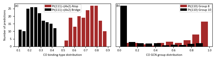
PLot all predictions for binding-types and GCN grups with large error

G = gridspec.GridSpec(1, 2)
CNCO_c4x2 = np.array(NN_CNCO.PREDICTIONS_LIST)[:,0,:]
GCN_p1x2 = np.array(NN_GCN.PREDICTIONS_LIST)[:,2,:]
plt.figure(1,figsize=(7.2,2))
ax1 = plt.subplot(G[0])
ax1.hist(CNCO_c4x2[:,0],bins=10,align='mid',rwidth=0.8,color='brown',zorder=1)
ax1.hist(CNCO_c4x2[:,1],bins=10,align='mid',rwidth=0.8,color='black',zorder=2)
ax1.legend(['Pt(111) c(4x2) Atop','Pt(111) c(4x2) Bridge'])
ax1.text(0.004,0.93,'(a)', transform=ax1.transAxes)
plt.xlabel('CO binding-type distribution')
plt.ylabel('Number of predictions')
ax2 = plt.subplot(G[1])
ax2.hist(GCN_p1x2[:,7],bins=10,align='mid',rwidth=0.8,color='brown',zorder=1)
ax2.hist(GCN_p1x2[:,9],bins=10,align='mid',rwidth=0.8,color='black',zorder=2)
ax2.legend(['Pt(110) Group 8','Pt(110) Group 10'])
ax2.text(0.004,0.93,'(b)', transform=ax2.transAxes)
plt.xlabel('CO GCN group distribution')
plt.yticks([])
plt.show()

Out:

C:\Users\lansf\Box Sync\Synced_Files\Coding\Python\Github\jl_spectra_2_structure\examples\predict_experiment\plot_predict_experiment.py:134: UserWarning: Matplotlib is currently using agg, which is a non-GUI backend, so cannot show the figure.
  plt.show()