Wasserstein loss and its derivative used in jl_spectra_2_structure

This example shows how to deconvolute spectra using the model

The parity plot for the mixtures where concentrations are known is shown in figure 1 and the plot of concentration with time for the experimental spectra from reacting systems are shown in figure 2 and 3 for different starting concentrations

import numpy as np
from scipy.special import kl_div
import matplotlib.pyplot as plt
from matplotlib import gridspec
from jl_spectra_2_structure.plotting_tools import set_figure_settings

set figure settings

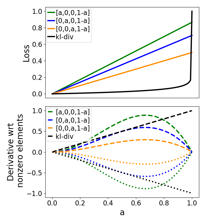
First we’ll set up vectors to store the wasserstein loss of A1, A2, and A3, with respect to B. The kl-divergence loss does not change with these threee vectors. Second we’ll set up the vectors to store the derivative of the loss with respect to the non-zero indices.

set_figure_settings('presentation')
a = np.linspace(0,1,num=100,endpoint=True)
B = [0,0,0,1]
Wl = np.zeros_like(a)
Wl2 = np.zeros_like(a)
Wl3 = np.zeros_like(a)
KL = np.zeros_like(a)
dEdO1 = np.zeros_like(a)
dEdO2 = np.zeros_like(a)
dEdO3 = np.zeros_like(a)
dEdO14 = np.zeros_like(a)
dEdO24 = np.zeros_like(a)
dEdO34 = np.zeros_like(a)
dKLdOi = np.zeros_like(a)
for i in range(len(a)):
    A = np.array([a[i],0,0,1-a[i]])
    Akl = [a[i]+10**-12,+10**-12,+10**-12,1-a[i]+10**-12]
    Bkl = [10**-12,10**-12,10**-12,1+10**-12]
    KL[i] = np.sum(kl_div(Bkl,Akl))
    dKLdOi[i] = a[i]
    W = (1/len(A)*np.sum((np.cumsum(A)-np.cumsum(B))**2))**0.5
    dEdO = 2*A*(np.cumsum((np.cumsum(A)-np.cumsum(B))[::-1])[::-1]-np.sum(np.cumsum(A)*(np.cumsum(A)-np.cumsum(B))))
    dEdO1[i] = dEdO[0]
    dEdO14[i] = dEdO[3]
    Wl[i]= W
    A = np.array([0,a[i],0,1-a[i]])
    W = (1/len(A)*np.sum((np.cumsum(A)-np.cumsum(B))**2))**0.5
    dEdO = 2*A*(np.cumsum((np.cumsum(A)-np.cumsum(B))[::-1])[::-1]-np.sum(np.cumsum(A)*(np.cumsum(A)-np.cumsum(B))))
    dEdO2[i] = dEdO[1]
    dEdO24[i] = dEdO[3]
    Wl2[i]= W
    A = np.array([0,0,a[i],1-a[i]])
    W = (1/len(A)*np.sum((np.cumsum(A)-np.cumsum(B))**2))**0.5
    dEdO = 2*A*(np.cumsum((np.cumsum(A)-np.cumsum(B))[::-1])[::-1]-np.sum(np.cumsum(A)*(np.cumsum(A)-np.cumsum(B))))
    dEdO3[i] = dEdO[2]
    dEdO34[i] = dEdO[3]
    Wl3[i]= W

KL/= np.max(KL)
G = gridspec.GridSpec(2, 1)
plt.figure(0,figsize=(7,7.6))
ax1 = plt.subplot(G[0,0])
ax1.plot(a,Wl,'g',a,Wl2,'b',a,Wl3,'darkorange',a,KL,'k')
plt.xticks([])
plt.ylabel('Loss')
plt.legend(['[a,0,0,1-a]','[0,a,0,1-a]','[0,0,a,1-a]','kl-div'])
ax2 = plt.subplot(G[1,0])
ax2.plot(a,dEdO1,'g--')
ax2.plot(a,dEdO2,'b--')
ax2.plot(a,dEdO3,'darkorange',linestyle='--')
ax2.plot(a,dKLdOi,'k--')
ax2.plot(a,dEdO14,'g:')
ax2.plot(a,dEdO24,'b:')
ax2.plot(a,dEdO34,'darkorange',linestyle=':')
ax2.plot(a,-dKLdOi,'k:')
plt.xlabel('a')
plt.ylabel('Derivative wrt\n nonzero elements')
plt.legend(['[a,0,0,1-a]','[0,a,0,1-a]','[0,0,a,1-a]','kl-div'])
plt.show()

Out:

C:\Users\lansf\Box Sync\Synced_Files\Coding\Python\Github\jl_spectra_2_structure\examples\wasserstein_loss\plot_wasserstein.py:86: UserWarning: Matplotlib is currently using agg, which is a non-GUI backend, so cannot show the figure.
  plt.show()